

A planner’s checklist: What telematics data can (and can’t) do for freight planning
Telematics data for freight planning complements traditional sources. Our checklists share what telematics data can and can’t do to support freight planning.


Origin-Destination (O/D) studies are the backbone of commercial transportation analytics, providing insights into three main types of transportation questions. But it’s not always obvious which type of O/D study to use for various scenarios, so planners often waste time running query after query to fine-tune the parameters.
To help planners match their study objective to the right view of O/D data, we offer several recommendations for reducing wasted query time on transportation studies.
To begin with, think about the questions each type of O/D analysis answers. This question-first framing helps planners choose the right analysis type before they dig into parameters.
How much freight moved between Zone A and Zone B? Closed O/D captures counts for commercial travel between one origin zone and one destination zone — for example, travel between a port and a warehouse. The zones can be counties, cities, Transportation Analysis Zones or custom polygons. Closed O/D data can be used for freight-demand studies, O/D matrices and infrastructure investment decisions.
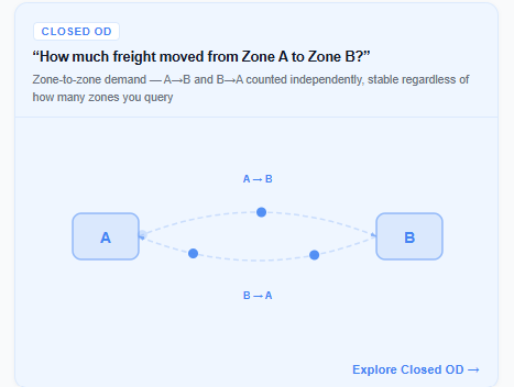
Figure 1: Closed O/D studies show freight travel movements between zones.
How much traffic used this highway corridor? Segment flow collects travel through a specific “gate” (like how many trucks take a certain bridge or toll road section) matching O/D pairs to show travel patterns through that gate. This data informs corridor flow, highway capacity, EV charging siting, toll road revenue and freight route designation.
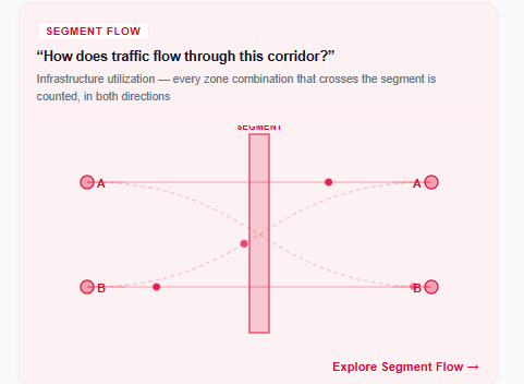
Figure 2: Segment flow analysis reveals how much commercial traffic flows through a particular corridor.
What’s all the traffic around this zone? Open O/D measures movements around an anchor zone to help planners understand all trips that begin in, end in or pass through that defined zone. The zone could be a city, a county, an industrial area, warehouse district or other area of interest.
The key difference from Closed O-D: you don’t need to define both origins and destinations upfront. Open O/D lets you discover where traffic is coming from or going to, which is useful for site analysis and catchment studies.
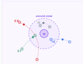
Open O/D trips fit into four zone flow types:
Here’s where O/D analysis can get tricky: Setting up the parameters. If you make a mistake defining the analysis logic, you can miss data or get inaccurately inflated counts. For example, without a minimum trip distance filter, an analysis of freight moving through an industrial corridor could also capture trucks repositioning between loading bays or staging areas. That would inflate your trip count without adding useful route data.
Here are some helpful tips for getting it right the first time, and reducing wasted query time on O/D transportation studies.
Trip pairing is critical. Capturing single trips creates highly variable data which is not a reliable demand indicator. To show aggregate travel patterns, O/D information must be captured as paired trips. Altitude’s platform sets pairwise attribution as the default behavior to ensure trip pairing.
Trip chaining defines the length of time a truck can stop (while delivering or refueling, for example) while still being considered a single trip. These are usually expressed by two parameters: MaxStopDuration (how long a vehicle can stop and still be counted as one journey) and ShortJourneyDistanceThreshold (minimum distance to filter out noise).
Setting a stop duration of 60 minutes means that a truck that stops for less than an hour and then continues still counts as one trip. A truck that stops for over an hour and then continues will count as two trips. If it stops again for longer than an hour, that’s three trips.
Figure out your trip chaining parameters before creating your analysis so you can input the correct data. A platform like Altitude’s with automated criteria for trip chaining removes obvious short trip breaks (like freight yard movements and fuel stops) creating more accurate trip counts.
Trip distance settings can filter out very short movements — for example, trucks moving around in freight yards, parking lots or loading docks. Or, for a segment flow, you may want to remove very long trips to focus on regional or metro travel. Decide ahead of time what distances you can filter out for more efficient analysis times and data tables.
In addition to trip counts, you may want to study metrics (like trip distance, trip duration or trip speeds) by day of week or time of day. Trip counts can also be split into vehicle types or vehicle vocations including:
Plan ahead to add these criteria on the first analysis instead of running multiple queries later to add attributes.
Look for more data in addition to weight class. For example, Altitude’s vehicle attributes include vocation (Long Haul, Regional, Drayage, etc.), fuel type and industry codes. These can be key differentiators for freight analysis.
For segment analysis, this parameter has three values: “false” (trips that stopped), “true” (stopped or passed through), “only” (pure through-traffic). This is a major efficiency lever for filtering local vs. long-haul traffic.
Being able to mix zone types allows you to ask questions like, “Where does traffic on I-85 come from and where does it go?” Getting the answer requires mixing infrastructure (segments) with geography (zones) in a single analysis.
For example, Altitude’s Segment Flow’s O-C-D (Origin-Connector-Destination) framework lets you combine area zones (counties, TAZs, custom polygons) as origins/destinations with road segments as connectors.
Learn more about studying movements between standard zones, custom zones or road segments with Altitude’s Origin & Destination analytics.
Start with your core question. If you need to measure freight movement between two known locations, Closed O/D is your best fit. If you’re exploring travel patterns around a site without a predetermined destination, Open O/D gives you more discovery flexibility. If your question is about traffic volume through a specific road or corridor, Segment Flow is the right choice. When in doubt, define your question before you define your zones.
Accuracy depends largely on the size and representativeness of the underlying GPS sample. Look for large, continuously updated datasets that apply data expansion methods to account for vehicles not directly observed. Make sure results are validated against known counts — like traffic monitoring stations — when using O/D data for major investment decisions.
Most O/D platforms support a range of zone sizes, from large regions like states and counties down to custom polygons around a single facility or intersection. Smaller zones produce more granular results but may require larger data samples to return statistically reliable counts. Match your zone size to the scale of the decision you’re making.
Yes, and it’s one of the most valuable applications for long-range transportation planning and grant documentation. Running the same study parameters across multiple years can reveal shifts in freight patterns, emerging corridors, or changing land use impacts — provided the platform maintains consistent historical data.
O/D analysis handles cross-jurisdictional movement well since it tracks trips from origin to destination regardless of how many county or state lines they cross. The key is defining your zones to capture the full extent of the travel pattern you’re studying, rather than limiting your analysis to a single jurisdiction boundary.
Most platforms export O/D results as CSV or Excel files for use in spreadsheets and travel demand models, and as shapefiles or GeoJSON for GIS platforms. If you’re integrating O/D data into a regional travel demand model, confirm that the trip table format is compatible with your modeling software before running your analysis.
Telematics data for freight planning complements traditional sources. Our checklists share what telematics data can and can’t do to support freight planning.
New data sources for MPO freight planning: 3 overlooked metrics that reveal regional trends before they hit your dashboard.
State DOTs can forecast truck traffic earlier by watching freight metrics from city and port data. Here are 3 signals worth tracking.